On a roll: An experiment in dice rolling

Abstract:

In this lab experiment it was conducted a simulation of dice rolls that determined that middle sums appear more frequently than those in the extremes, it was also noted that the frequency created a bell-Shaped curve resembling an standard deviation curve

Introduction

Probability is a fundamental concept that rules over many things in our world that can help in predicting the likelihood of the outcome in random events. This lab will focus on measuring the probability distribution of the rolling of two six-sided dice, and when rolled together the outcome can range from two to twelve. The purpose of this experiment will be to calculate the probability of each independent outcome and measure the likelihood of each outcome.   The leading hypothesis for this experiment is that outcomes ranging in the middle of two to twelve, meaning six, seven, and eight. Will be more likely to appear than extreme values like two or twelve. This is based upon the greater amplitude of combination that can produce middle sums, it can also be predicted that the data from the experiment will form a standard deviation graph

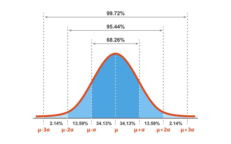Figure 2.1 A visualization of a standard deviation graph

The reason for this experiment is that it can provide the chance to put theoretical probabilities to the test in a real-world experiment. Also, this experiment will help us understand how the number of possible combinations can influence the likelihood of a specific sum, where middle values like six, seven, and eight are expected to occur more often than the extremes two or twelve.  

Materials and Methods

Materials

• Computer with python installed
• Provided script: Dice roll
• Microsoft excel (or any other spreadsheet software)

Methods To proceed with the experiment the Python script Dice roll was used to simulate the rolling of two six-sided dice. The program was executed with python software, the one used for this experiment was PyCharm. After executing the script, the user is then prompted to input the desired number of rolls, 5,000 rolls were used for this experiment. The script then simulated the rolls, thus generating a random number between one and six, for every roll the script recorded the results of each individual die and the sum of the two. This data was then automatically collected into a CSV file with the title dice_rolls.cvs, that was stored in the same directory as the script. When the simulation was completed the CSV file was opened in the Excel to be able to organize and analyze the data. The data columns were labeled by the script as roll, die 1, die 2, and sum the roll collum was omitted for this experiment. After a frequency table using the function frequency() was created to determine how many times each possible sum, ranging from two to twelve, occurred during the simulation. Then the probability of the sums was calculated by dividing the frequency by the total number of trials (5,000). To give a visualization of these results a bar chart was created using the calculations, finally the graph was analyzed to determine whether or not it resembled a standard deviation curve, thereby supporting or refuting the hypothesis that the middle sums would occur more frequently than the extremes.       Results The dice rolling simulation was conducted for 5,000 rolls, with each roll involving two six-sided dice. The recorded rolls included the individual results of each die and their combined sum. The frequency of each possible sum was calculated and their respective probability. The most frequent outcomes were the middle sums. The sum of 7 occurred most frequently, appearing 560 times and accounting for 11.20% of the total rolls. Other sums near the middle, such as 6 and 8, had high frequencies as well, with 416 and 428 occurrences, corresponding to 8.32% and 8.56% of the rolls, respectively. As a contrast, the extreme sums, such as 2 and 12, were less frequent, appearing 144 and 145 times, respectively, both representing approximately 2.88% of the total rolls.

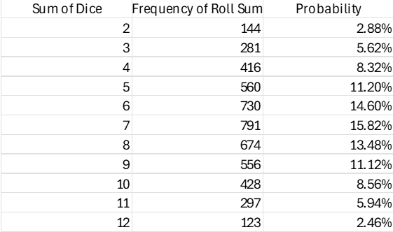Figure 3.1 Table of the frequency and probability of each sum

A bar chart was generated to visualize the frequency distribution of the sums. The chart displayed a bell-shaped curve, with higher frequencies concentrated around the middle sums and lower frequencies at the extremes.

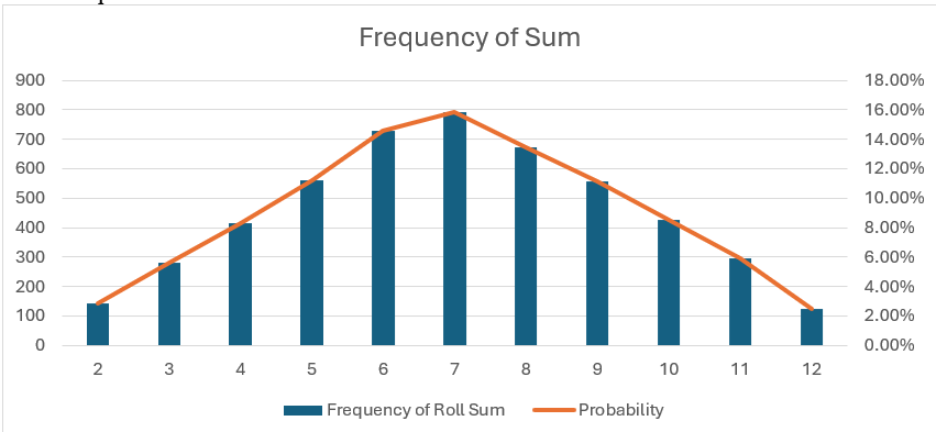
Figure 3.2 graphic representation of the table

Analysis The experimental results of the 5,000 simulated dice rolls demonstrated a frequency distribution consistent with the theoretical expectation of the rolling of two six-sided dice demonstrated that middle sums, such as six, seven, and eight, occurred more frequently than the extremes two and twelve. These results align with the nature of numbers with more possible combination are statistically more likely. Baker (2013) argues that “Understanding that there is a 1/6 chance of rolling any given number on a fair six-sided die is fairly intuitive” (Baker, 2013, p. 1), but “probabilities change when a second die is added; each outcome between the upper and lower limits then has multiple ways of being rolled” (Baker, 2013, p. 1). This concept can directly relate to the results found during the experiment, where the sums in the middle of the range were more frequent than those in the extremes due to the larger amount of combinations possible to produce them Furthermore, the experiment’s results support Baker’s discussion of probability distributions in dice rolling. He notes that “as more dice are added, the standard deviation of the data set drops in relation to its total width. Outcomes at both extremes become rarer, whereas the most probable outcomes cluster more around the center” (p. 555)​. In this case, while only two dice were used, the pattern still demonstrated this trend, reinforcing the relationship between probability distributions and randomness in dice rolls.

Conclusion

Overall, the experiment validated the hypothesis that middle sums would occur more frequently. The frequency distribution and calculated probabilities reflected expected trends, with minimal deviations, demonstrating the practical value of simulations for understanding probability and randomness.     References Baker, J. D. (2013). Delving deeper: rolling the dice. Mathematics Teacher Learning and Teaching PK-12, 106(7), 551–556. https://doi.org/10.5951/mathteacher.106.7.0551 Fig1.1 was generated with an AI program using the prompt “generate an image of 2 dice being rolled” Figure 2.1 was collected from the website https://www.freepik.com/premium-vector/gauss-distribution-standard-normal-distribution-gaussian-bell-graph-curve-business-marketing-concept-math-probability-theory-editable-stroke-vector-illustration-isolated-white-background_26381152.htm         Appendix Dice roll script: import random import csv def roll_dice(): die1 = random.randint(1, 6) die2 = random.randint(1, 6) total = die1 + die2 return die1, die2, total def main(): try: rolls = int(input(“Enter the number of times you want to roll the dice: “)) except ValueError: print(“Invalid input. Please enter an integer.”) return with open(‘dice_rolls.csv’, ‘w’, newline=”) as file: writer = csv.writer(file) writer.writerow([‘Roll’, ‘Die 1’, ‘Die 2’, ‘Sum’]) for i in range(1, rolls + 1): die1, die2, total = roll_dice() writer.writerow([i, die1, die2, total]) print(f”{i:<5}{die1:<10}{die2:<10}{total:<5}”) print(“\nData has been saved to ‘dice_rolls.csv’.”) if __name__ == “__main__”: main() Complete Dataset: dice_rolls.xlsx